This post builds on top of this article from Towards Data Science: https://towardsdatascience.com/explaining-feature-importance-by-example-of-a-random-forest-d9166011959e. Here I talk about the column drop method, which evaluates the performance of the classifier with one feature removed. For some reason, the article above computes the benchmark score with all features on the same training dataset, and it does not use cross-validation to compute the margin of error.
I have adapted the code from the article to compute all the scores with cross-validation and then draw a boxplot with errors:
import pandas as pd
from sklearn.base import clone
from sklearn.model_selection import StratifiedShuffleSplit, cross_val_score
def drop_col_feat_imp(model, X, y, random_state=None):
# clone the model to have the exact same specification as the one initially trained
model_clone = clone(model)
# set random_state for comparability
model_clone.random_state = random_state
# training and scoring the benchmark model
cv = StratifiedShuffleSplit(n_splits=10, test_size=0.2, random_state=random_state)
benchmark_score = cross_val_score(model_clone, X, y, cv=cv, scoring="f1", n_jobs=-1)
# list for storing feature importances
importances = []
# iterating over all columns and storing feature importance (difference between benchmark and new model)
for col in X.columns:
model_clone = clone(model)
model_clone.random_state = random_state
drop_col_score = cross_val_score(model_clone, X.drop(col, axis = 1), y, cv=cv, scoring="f1")
score_diffs = benchmark_score - drop_col_score
for score_diff in score_diffs:
importances.append({'score_diff': score_diff, 'feature': col})
importances_df = pd.DataFrame(importances)
return importances_df
importances = drop_col_feat_imp(model, X, y)
def boxplot_sorted(df, by, column):
temp_df = pd.DataFrame({col:vals[column] for col, vals in df.groupby(by)})
meds = temp_df.median().sort_values()
temp_df[meds.index].boxplot(vert=False, figsize=(10,6))
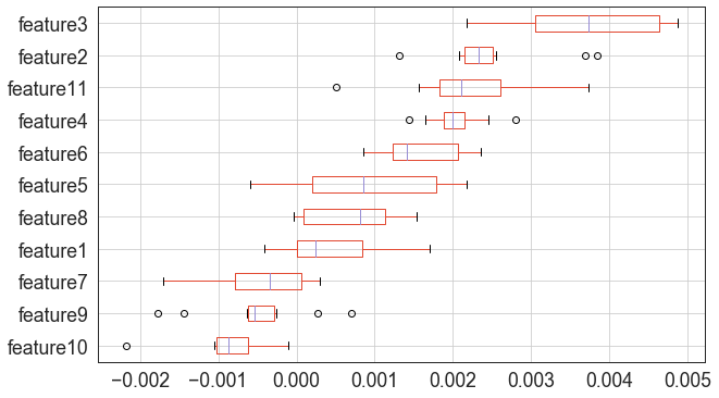
boxplot_sorted(importances, by=["feature"], column="score_diff")In the end you should see a graph similar to the following: